My Pathtracing Journey: Part 1

Hello again :). I think the best way to kick off this blog is with a devlog!

In this series of a couple blog posts I will be documenting the development process of my latest graphics project: a simple offline unidirectional pathtracer, that works on the CPU. This is one of the bigger codebases I’ve worked on, and as a student, that isn’t really saying much as it is still fairly small. The full project is viewable on GitHub, here.

The theory

As anyone that has ever implemented a simple pathtracer will tell you, it’s extremely simple to start out such a project and have a pretty picture on the screen, but it gets difficult to go past that, without knowing what you’re doing. Having already implemented a simplistic pathtracer, following the lead of Peter Shirley’s amazing book “Raytracing in One Weekend” (which you can find here), I got pretty good results, but was unsure what to do, as I hadn’t actually learnt anything about how light travels throughout the scene.

I had heard about a few books on the topic of light transport, mainly “Physically Based Rendering: From Theory to Implementation”, and “Advanced Global Illumination” and had planned to get around to reading them. At the time, in the Graphics Programming Discord (a Discord server full of amazingly talented graphics programmers, which you can visit using this invite link), a couple users were organizing a collaborative reading and discussion session on the book “Advanced Global Illimunation”. These sessions were amazing and have really helped me fill in the holes in my maths understanding. (A special thanks to Criver, Jaker, Zuen, Legend and many more, for dealing with my many many questions ❤️)

After taking my time with learning the theory and the math behind it, I felt more comfortable with concepts such as radiometric quantities, radiance, the rendering equation, bidirectional reflectance distribution functions, acceleration structures, and a lot more. I could finally understand what concepts were being used in Peter Shirley’s simple but amazing implementation of a pathtracer.

Implementation

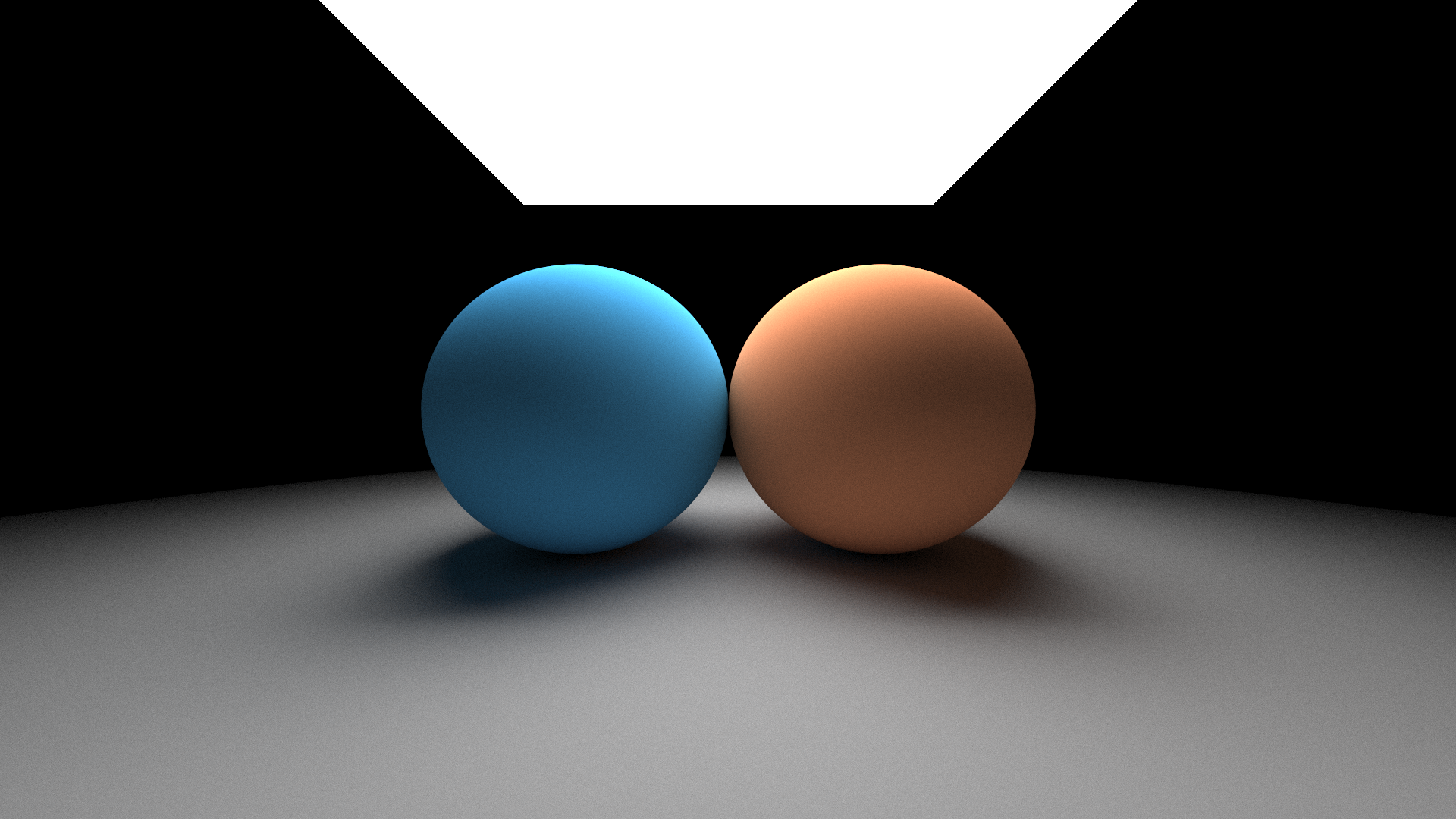
To test out my knowledge, I tried to create a pathtracer from scratch, using the general outlined steps used to measure the flux for a given pixel grid, described in the book. I managed to implement a simplistic Lambertian BRDF, and using hemisphere sampling on each bounce with no importance sampling of any sort, rendered my first scene!

I got these results while following Peter Shirley’s book as well, but now it was different. I could reason and actually understand why and how the light energy propagated thoughout the scene! I am certainly not at a level that I could derive the actual equations, but understanding them intuitively has helped immensely.

Next up, I wanted to render the legendary Cornell Box, used by many graphics researchers in the early years of the field. I still didn’t have third-party model support, so I cobbled together a scene built with the primitives I had implemented. But, with such a scene, even the small amount of triangles I had slowed down the rendering time.

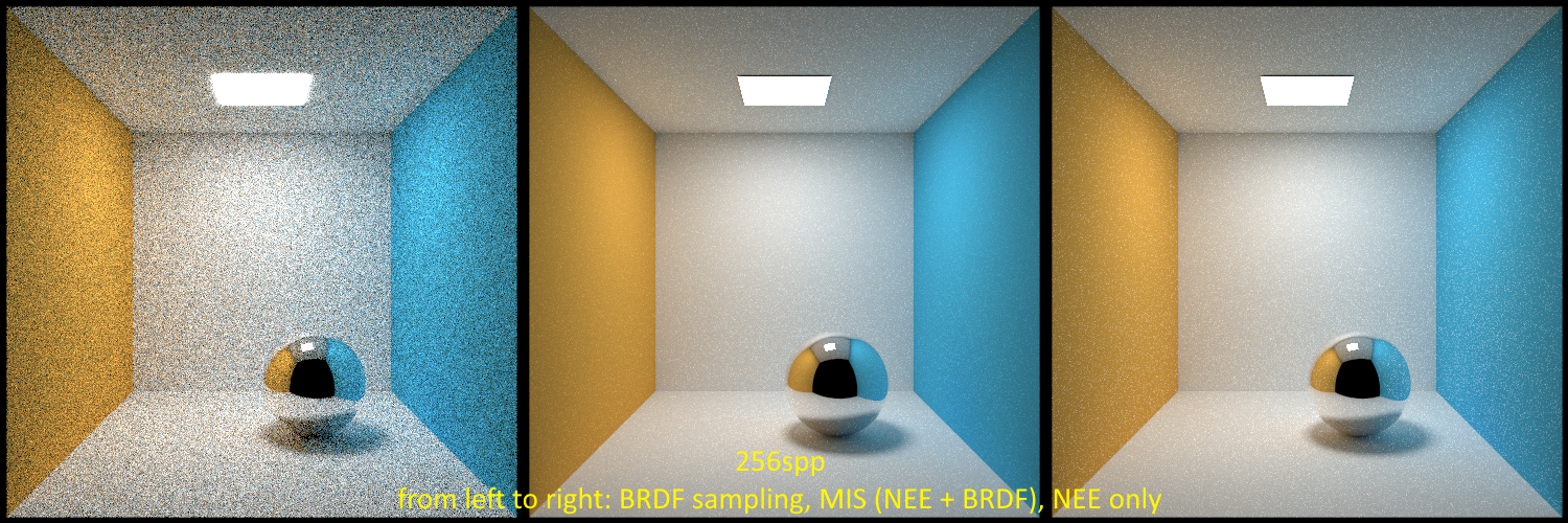
Wanting to have quicker render times with smaller sample counts, I decided to try out Next Event Estimation (a method where the direct illumination is calculated on each bounce and accumulated, instead of when a ray hits the light source). With this variance reduction method, the rays that would otherwise bounce around the scene but not hit the light source, instead of contributing 0 energy to the calculations, were taken into account. This practically resulted in a decrease in noise in the final result.

Implementing a purely specular BRDF in the scene (shown on the sphere in the above image), resulted in some fireflies in the NEE result. As a saving measure, I implemented Multiple Importance Sampling (MIS) as a method to combine 2 or more integral estimators such that, whenever one estimator contributes more than the others, that one is picked with a higher weighing coefficient. Using the balance heuristic between the brute-force hemisphere sampling estimator and the NEE estimator, I got less noise and fewer fireflies in the final result! The above image shows a comparison of the three estimators.

Implementing mesh support (using the amazing OBJ model loading library TinyOBJLoader) opened up the gates to test out many different simple and complex meshes! I implemented partial support for the OBJ material format, using the Modified Blinn-Phong BRDF which should be more truthful and physically-based than the Phong BRDF. This scene was quick enough to render, although I could feel the extreme slowdown when tried out even simple meshes.

As a method to speed up rendering time, I figured I would implement a thread-pool, with threads waiting to render parts of the image. The general rule of thumb I had heard up until that point was to split the image into chunks of 32x32 or 64x64 pixels, and to assign a thread to each chunk. I used Win32 native threads and Linux POSIX threads for the job, as the purpose of the thread-pool didn’t necessate usage of a more complex third-party library for the job. The speedup was tremendous! What took an hour and more before, now took a few minutes!

A few minutes at the time felt like a major speedup, although this was while using low-poly meshes, with each triangle from the mesh being tested against for each ray that got shot at the virtual screen. If we do the math, 1920x1080 pixels, ~200 samples per pixel, 5 ray bounces on average, that is close to 2 billion rays that need to test if they are interesecting with each and every single triangle in the scene! It was time to implement an acceleration structure…

There are some amazing Bounding Volume Hierarchy (BVH) construction and traversal libraries out there, even hardware implementations exist with the newer raytracing-capable graphics cards! But, in order to understand what a BVH does internally, I wanted to implement one myself. In the beginning, I used a triangle-median node splitting heuristic that resulted in each node getting split into equally-sized disjoint sets of triangles, sorted along a random 3D axis. This had good results and sped up my rendering time significantly, resulting in a few minute render time drop!

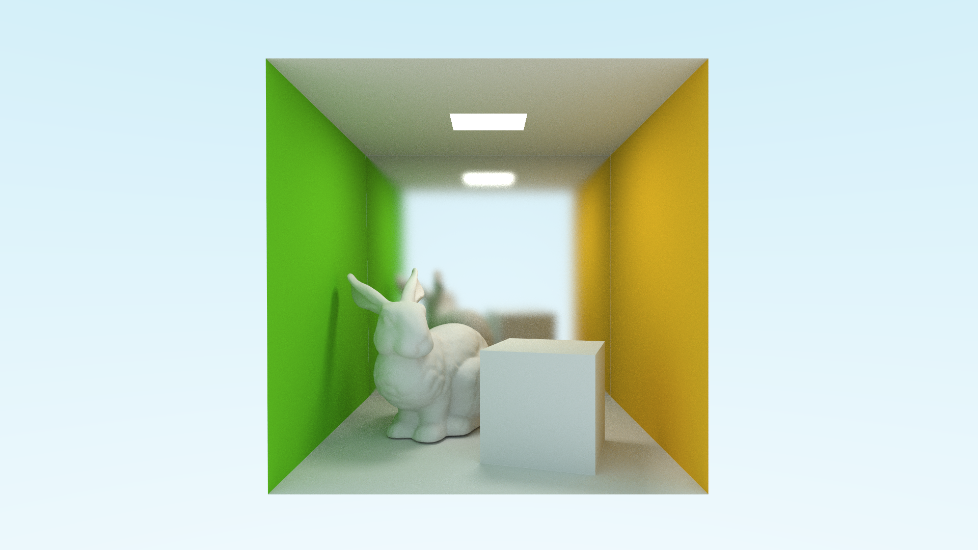
I could finally render a more complex model such as the Stanford Bunny shown in the above render. The bunny mesh has a significant polygon count, resulting in a total render time of about 5 minutes (40-50 minutes without a BVH). Furthermore, I implemented the Surface Area Heuristic (SAH) for deciding how to split each node. This resulted in a small speedup up to 3 minutes in render time (accounting for BVH building time). Smaller meshes with a couple of thousand triangles are rendered in the order of tens of seconds, which I think is good enough for my purposes, for now!

What next?

The time I’ve allocated to this project has varied significantly over the past year as I have been busy with my university studies, but I have not given up on working on it!

I plan to work on more variance reduction techniques in order to use a smaller sample count to achieve similar results to what I now achieve with a large sample count. I would like to implement more advanced BRDFs and to fully support any OBJ model I find on the Internet, along with its material (with possible GLTF model support in the further future). Ultimately, I would also move the project over to the GPU, in order to achieve real-time performance, along with a controllable 3D camera! This could either be through a fullscreen tri and fragment shader, or a compute shader.

Thank you for reading my little journey (so far). If this post was interesting to you, make sure to be around for my next posts covering the upcoming features! This blog has a functioning RSS feed to use in your favorite RSS reader :)